image source

Data science and Machine learning have become buzzwords that swept the world by storm. They say that data scientist is one of the sexiest job in the 21st century, and machine learning online courses can be found easily online, focusing on fancy machine learning models such as random forest, state vector machine and neural networks. However, machine learning and choosing models is just a small part of the data science pipeline.

This is part 3 of a 4 part tutorial which provides a step-by-step guide in addressing a data science problem with machine learning, using the complete data science pipeline and python pandas and sklearn as a tool, to analyse and covert data into useful information that can be used by a business. The previous parts of the tutorial can be found here:

Part 1
Part 2

In this tutorial, I will be using a dataset that is publicly available which can be found in the following link:

https://archive.ics.uci.edu/ml/datasets/BlogFeedback

Note that this was used in an interview question for a data scientist position at a certain financial institute. The question was: whether this data is useful. It’s a vague question, but it is often what businesses face – they don’t really have any particular application in mind. The actual value of data need to be discovered.

The third tutorial will be covering the third steps in the pipeline: Apply and evaluating a machine learning model to the data.

Recap

We have loaded in this dataset into the following dataframes:

df_stats: Site Stats Data (columns 1 – 50)
df_total_comment: Total comment over 72hr (column 51)
df_prev_comments: Comment history data (columns 51 – 55)
df_prev_trackback: Link history data (columns 56 – 60)
df_time: Basetime - publish time (column 61)
df_length: Length of Blogpost (column 62)
df_bow: Bag of word data (column 63 – 262)
df_weekday_B: Basetime day of week (column 263 – 269)
df_weekday_P: Publish day of week (column 270 – 276)
df_parents: Parent data (column 277 – 280)
df_target: comments next 24hrs (column 281)

We understand quite a bit of what the data is telling us, through visually inspecting the data and simple statistical analysis. We have already made some conclusions and suggestions without machine learning, but now it's time to unleash the full power of the data through machine learning.

Framing the problem and the ML Pipeline

Similar to all problems, it is important to know what we are trying to solve before diving into the data. As pointed out in the last tutorial, our problem at hand is trying to predict posts that will be popular in the next 24 hours, in order to ensure the company’s presence on these posts. To do that, just like last tutorial, we could define if the number of comments exceeds 50 in the next 24 hours, the post is consider popular. The problem therefore can be framed as a classification problem: we are going to use machine learning and the data available to classify whether a post is going to be popular, or not.

After defining the problem, all machine learning problems follow the same pipeline: data preprocessing, choosing and training the model, apply model to test data and evaluate the performance with chosen metrics, and then repeat and adjust the model until the desired performance is achieved. Once that's reached, the model can then be launched or taken online, i.e. used to predict real data.

Data preprocessing

Data as is is often unfit for putting into a machine learning problem, and so data preprocessing is necessary. For this set of data, we have already performed some data preprocessing, such as removing duplicate columns and removing or filling in missing data in the first tutorial. We would also need to, for this dataset, to convert df_target into Boolean as we have done in the previous tutorial such that we have a classification problem:

The column df_target[‘target_clf’] now becomes the target labels for our classification problem. I am also going to specify here that for the reduction of computation time, I am only going to use a subset of the 281 column available. This decision was made as a trade-off for computation time, and the fact that a lot of the columns are dependent columns. For example, the first 50 columns are the statistics of the columns 51- 60, which means that columns 51-60 should contain all information the is needed. Some of these decisions can also be made based on experience and instinct. There are techniques which can be used to determine the dependency of different column (eg PCA), but this is outside the scope of this tutorial. Instead, I will just state here that the following dataframe are picked for the machine learning model, and merged into a master dataframe df_data:

Note how for some dataframes the whole dataframe is used, whereas for others only selected columns are used. You can check out the new dataframe with head():

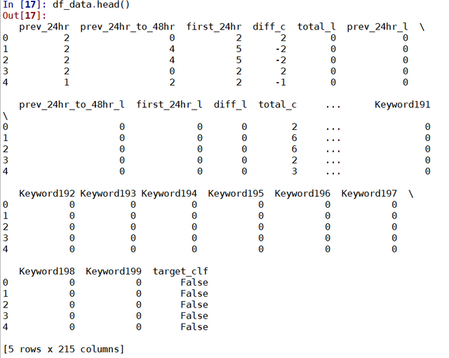
Again, if computational power or time is not a factor, by all means use all the data available. The next step in data preprocessing is splitting the data into a training set, cross validation set and test set. By definition, the training set is used to train the machine learning model, and the test set is used to assess the performance of the model. This is needed because if one judge the performance of the model with the same dataset that is used to train the model, optimisation process would improve the model with respect to the training data only, and would fail to generalise to real data. This effect is called overfitting. This can be avoided by using a test dataset for evaluation. Now, if you also plan to do model parameters optimisation, then it is also best to have a cross validation data, which is solely use during the model optimisation process, to avoid overfitting to the test data. Essentially you are creating two sets of test datasets, one for optimising the model (the cross validation set), the other to evaluate the final optimised performance of the model (the test set).

For our problem here, the test data is actually provided as a separate dataset. Therefore, we would just need to split the data into two parts. sckit-learn provides a very easy way to split data into train and test set:

Whereby you can specify the X (data) and Y (target labels) and set the ratio between the train and cross-validation set sizes using test_size. Usually a 70:30 (test_size = 0.3) split or 60:40 (test_size = 0.4) split would be adequate. As you will notice, that would mean that we would have a reduced number of training samples. Since we are actually provided with a seperate test dataset, it might actually be better to split the test data into a test set and a cross-validation set. We can do this with the following custom function:

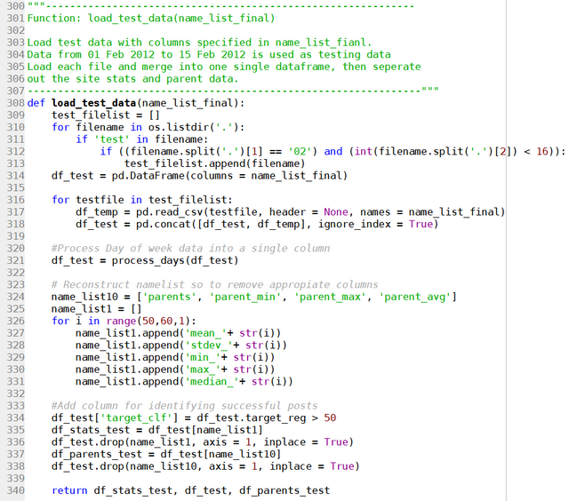
This function loads in all test data files from the first 15 days of Feb 2012 as the cross-validation data for optimising the model, and apply the same data preprocessing to this data as to the training data. Note that name_list_final contains the list of column names that was used for all 11 dataframe specified at the beginning. We can thus load the cross_validation data in df_test by:

Note the other processing required, such as reordering the columns and splitting the X and Y components of df_test.

Imbalanced Data

Recall that from statistical analysis in the previous tutorial, we have discovered that majority of the posts are actually not popular. This is expected, as only a few out of the many posts made on the internet is expected to be noticed by other users and become popular. So most of our data would have a target label of False. This is known as data imbalance. A big issue with imbalanced data is the difficulty in getting a good model as is. That is because the optimisation of a machine learning model is based on generating as many correct labels as possible. Consider an extreme case, where you only have 10 true labels in a pool of 100 samples. A model which simply says target equal False for all samples would be correct 90% of the time! Therefore, it is hard to optimise a model like this, as it will be dominated by the false samples. To solve this problem, the best approach is to add more data sample which have a True label. However, it may not be possible to do that in real life, as in this case here. An alternative approach is to synthesis data that have a true label. One way to do that is call bootstrap sampling, where we randomly select data samples in the positive dataset (with replacement) and duplicate it. It is counter intuitive, but it can be shown mathematically that this is equivalent to collecting more positive samples randomly in the real sample space (which is why it's called “bootstrap”, from the idea that you are pulling yourself higher by pulling on your bootstrap, which is in theory impossible). The following scripts can be used to perform bootstrapping:

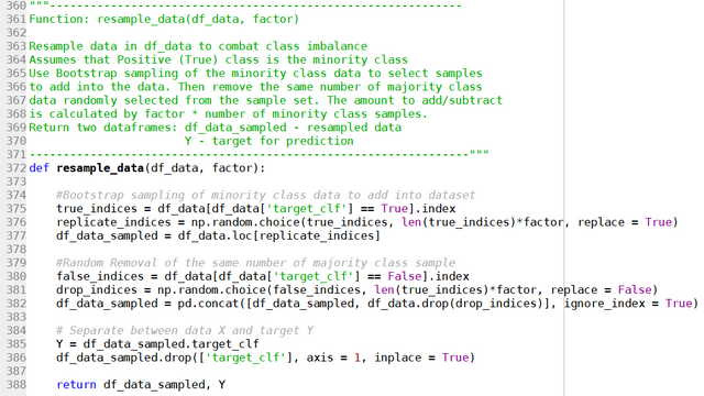
Note how I am also removing the same number of negative samples as the additional replicated positive samples, to increase the proportion of positive samples in the training data. Therefore, we can resample data by calling the function above:

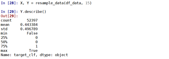
Using describe() we can see that the mean of Y is now close to 0.5, which means that the number of True and False samples are approximately equal. The total number of samples in the training set X remain unchanged.

This dataset is almost ready for model training. There are two things that I would like to mention. The first one is using categorical data. Recall that we have labelled the day-of-week columns into Monday to Sunday. We would need to convert this column, which currently is of the string type, into categorical data for a machine learning model to be applied. This can be easily done as follow using LabelEncoder():

Note how the same model is applied to both the training data and the cross-validation data. This ensures the two datasets have the same distribution. Another thing that may be necessary is performing scaling of data. This is especially important if an Eucliean based model (i.e. model based on optimisation through minimising distance data points) is used. The need of data scaling can be understood as follows: if you have two columns, one varies in the order of millions, one varies in the order of hundreds , then any variation in the first column is going to dominate the variation of your data, and therefore the final model will be skewed to that column. Data scaling using a column’s mean and standard deviation would solve this issue. Scaling can be done easily with the StandardScaler() function, for example:

However, with other models, e.g. decision tree models which is used here, scaling is not essential. Therefore, we are not going to scale our data in this tutorial. At this point, the data is ready for training our model.

Machine Learning Models

There are a lot of machine learning models out there. Some are targeted for certain applications and may have better performance in selected cases. However, for most cases, especially as a first try, choosing which model to use is not important, and they are most likely to give you a very similar result, as long as you do the data preprocessing correctly.

Having said that, there are models which in general performs slightly better than others and is often used by machine learning enthusiast, especially for data science competitions. Here, we will be using a model for gradient boosting, which is a powerful machine learning model that is natively implemented in scikit-learn.

Gradient boosting is a form of ensemble model known as boosting. Ensemble is a term that means that you are combining a bunch of less powerful models to get a more powerful model. And boosting is a method of doing that. In boosting, for each iteration, you generate a weak model (eg a simple decision tree), and then look at the data points that was not well predicted by the model, and put a emphasis on these data points (by giving them a higher weight), and train the next model. The next model would thus hopefully be targeted to predict these data points better. The process is iterated many times to generate a bunch of models that is then combined to predict all data points better. Boosting have been shown to be very powerful for numerical data problems. Gradient Boosting is just one type of boosting that uses the gradient descent optimisation algorithm to determine the weight of each successive model.

Training the model is in-fact the simplest part of the code. The gradient boosting model can be trained as follows:

Where the main parameters are n_estimators which specify how many simple models are used to form the complex model, and the learning_rate which specify how quickly the gradient descent optimises (A large learning rate would mean bigger optimisation step but also mean that it may not quite reach the local minima). These are hyperparameters that can be optimised to improve the performance of the model. Once the model is trained, we can use the model to make a prediction based on the data X_test. There are two ways to predict, either by predicting the actual class labels with predict(), or predicting the probability of a particular data point being in each of the class using predict_proba():

Evaluating the model performance

To evaluate the performance of a machine learning model, there are a number of metrics available. These metrics essentially are different ways to look at how different is the predicted value is compared to the ground truth in the cross validation or the test data. In this tutorial, we will be looking at two different metrics: the ROC AUC Score, and the confusion matrix.

The ROC AUC score is a matrix that looks at the Area Under the Curve (AUC) of the Receiver Operating Characteristic (ROC). The mathematical theory behind the ROC AUC is out of the scope of this tutorial. All we need to know is that if the model give a random number prediction, the ROC AUC score will be 0.5, whereas if the prediction is perfect, the AUC score will be 1. The ROC AUC score can be calculated with a built-in function:

The AUC Score is 0.946, which means the model is very good. The AUC score is a very handy one number metric for the performance of a model. In particular, it is a much better score to use than the accuracy, as the AUC score takes into account of the False Positives (see below).

The confusion matrix uses four different ways to look at the difference between the predicted labels and the ground truth. In particular, the confusion matrix contains four values: True data that have been correctly predicted as true (True Positives), True data that have been incorrectly predicted as False (False Negatives), False data that have been incorrectly predicted as True (False Positives), and False data that have been correctly predicted as True (True Negatives). The confusion matrix can be computed with the built-in function confusion_matrix():

It can be seen that for the model that we trained, True Positives are is much higher than False Negative, which means that the model had predicted True data very well: Out of the 36 cases of popular posts, we predicted 30 of them. So the model is doing reasonably well in predicting the correct posts - the Recall score (=30/36) is reasonable. However, we can also see from the confusion matrix that the number of false positive is very large: 132. This means that a lot of posts that are not going to be popular, actually will be predicted as popular. In this sense, the model is not very good at giving the right answer, in that most of the positive predictions are actually bad posts - the Precision Score (= 30/168) is low.

A slide presenting the results above that was prepared for the interview is attached:

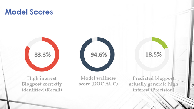
So which one of these are more important? Essentially, the model can pick out most of the posts that will become popular, but in the process also pick out a lot of posts that are not going to be popular. Is this model good enough for our application? It’s all and well that we applied a model and have a performance metric. But in order to really evaluate how the model will perform in real life, we need to think back to how we will use the predictions from the model. I will cover this as well as how we can improve our model in the next tutorial.

---

Posted on Utopian.io - Rewarding Open Source Contributors

---