R Programming Tutorial – How to Compute PI using Monte Carlo in R? R语言入门之 – 如何通过Monte Carlo来计算 PI?

 This tutorial will continue to help you understand how powerful R is to handle the vectors (arrays). 

 We know that the math constant  can be approximated by 4 times of the number of points inside a 1/4 circle divided by the total number of points. This is known as the Monte Carlo computation, which is to create as many random sample points as possible and count the statistics.   

set.seed(0.234234)

We can set the random seed by using set.seed() function (you can set to a constant number in order to reproduce the same ‘random’ data sets), e.g.: 

上次开始步入R语言的世界, 感觉R还是挺简洁强大的. 学一门程序最好的办法就是敲代码, 敲例子. 在工作生活中如果遇到需要敲代码的时候就得问问自己能否拿R语言来解决? 这样能更好的进步. 

 我们都知道圆周率可以通过随机在一个正方形(坐标X/Y均为0到1)撒足够多的点. 统计一下点在1/4的圆内(半径为1)的个数和总的撒点个数 这个值就会很接近 pi/4  . 因为圆的面积公式为    pi * r * r

 这种方法也称之为蒙特卡罗方法, 是一种随机, 统计的方法. 

 我们可以通过 runif 来生成随机的点, 参数指定点的个数,  

 Now, we can generate two vectors given a length, for example: 

x=runif(100000)

y=runif(100000)

 每个随机值是在0到1之间的浮点数(也可以指定 min=0,max=1). 然后可以把长度放在另一个向量里:  

 These random numbers are float numbers between 0 and 1, which can be visualized as 100000 points. So we can now compute their distance to the (0, 0), or the radius of the circle. 

z=sqrt(x^2+y^2)

 这时候我们只要统计出这个z数组里小于或等于1的个数即可. R语言里的 which 函数返回了数组里满足条件的 索引值, 那么我们只需要通过:  

 Now, z is also length of 100000. We next need to count how many of the distances in z vector are smaller than 1 (falling inside the 1/4 circle). We can use which to return all indices of the array given a condition. 

length(which(z<=1))

 即可以得到在圆内点的个数, 记得乘于4再除于样本的个数 就可以得到圆周率的近似值 (点数越多 精度越接近, 但  是个无理数)  

 To count the points, we use the length function. And the PI is finally estimated in a straightforward expression. Remember, this is just the approximation and the accuracy does improve when the number of samples gets larger and larger. 

length(which(z<=1))*4/length(z)

[1] 3.1454 

画图   PLOT THE POINTS

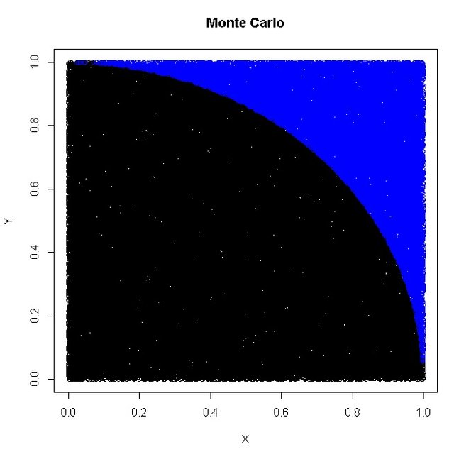
把在圆内的点画出来 (不指定颜色默认为黑色)  

 We can plot the points (that fall inside the circle) using (default black color if color is not specified): 

plot(x[which(z<=1)],y[which(z<=1)],xlab="X",ylab="Y",main="Monte Carlo")

 再把剩下的点用蓝色画出来 (注意这里用的是 points 方法在原来的图上画):  

 and points outside the circle (noted in blue color) can be added to the same plot using: 

points(x[which(z>1)],y[which(z>1)],col='blue')

 最后面就很直观的能解释这种算法.   This finally gives the plot: 

 You see? No for/while loops, just 4 statements in R! 

 这个例子中R非常强大, 没用到 for/while (Python, Matlab 也可以). 传统编程语言基本都是需要用到for或者while的. 从这个例子中是不是能看出统计学出生的R语言的一些编程风格呢? 

Thank you for reading my post, feel free to FOLLOW and Upvote @justyy, which motivates me to create more quality posts.  

根据我的博文  这篇 和 这篇 整理。 非常感谢阅读，欢迎FOLLOW和Upvote @justyy 能激励我创作更多更好的内容。