Sets of Julia
Hello to all the beautiful scientific community of Steemit, I want to show you an intuitive definition of Julia sets. This definition I develop in my research on basins of attraction of nonlinear equations in my university.
Sets of Julia.
These sets are the source of some of the most interesting and well-known fractals of the present time. In 1918 Gaston Julia, a French mathematician, published his works on these sets bearing his name. In addition to the other mathematicians like Pierre Fatuo, they promoted the progress of this research.
Julia sets are defined through polynomial iterations and functions defined in the complex plane.
If f (x) is a function, several behaviors arise when f is iterated, let us take for example the function:
f(x) = x^2 − 0,75
Consider x = a0 the initial point of the succession defined as:
a1 = f(a0)
a2 = f(a1) = f(f(a0))
.
.
.
an = f(a^n−1) = f(f· · · (f(a0))
.
.
.
It may be that the values of the infinite succession of iterations {ak: k ∈ N} are maintained bounded or not, but this will depend on the initial value a0.
Example: If we iterate f (x) = x ^ 2 - 0.75 taking as initial point a0 = 1 we obtain
the next:
A0 = 1
A1 = f (1) = 12 - 0.75 = 0.25
A2 = f (0.25) = 0.252 - 0.75 = -0.6875
A3 = f (-0.6875) = (-0.6875) 2 = 0.75 = -0.2773
A4 = f (-0.2773) = (-0.2773) 2 - 0.75 = -0.6731
A5 = f (-0.6731) = (-0.6731) 2 = 0.75 = -0.2970
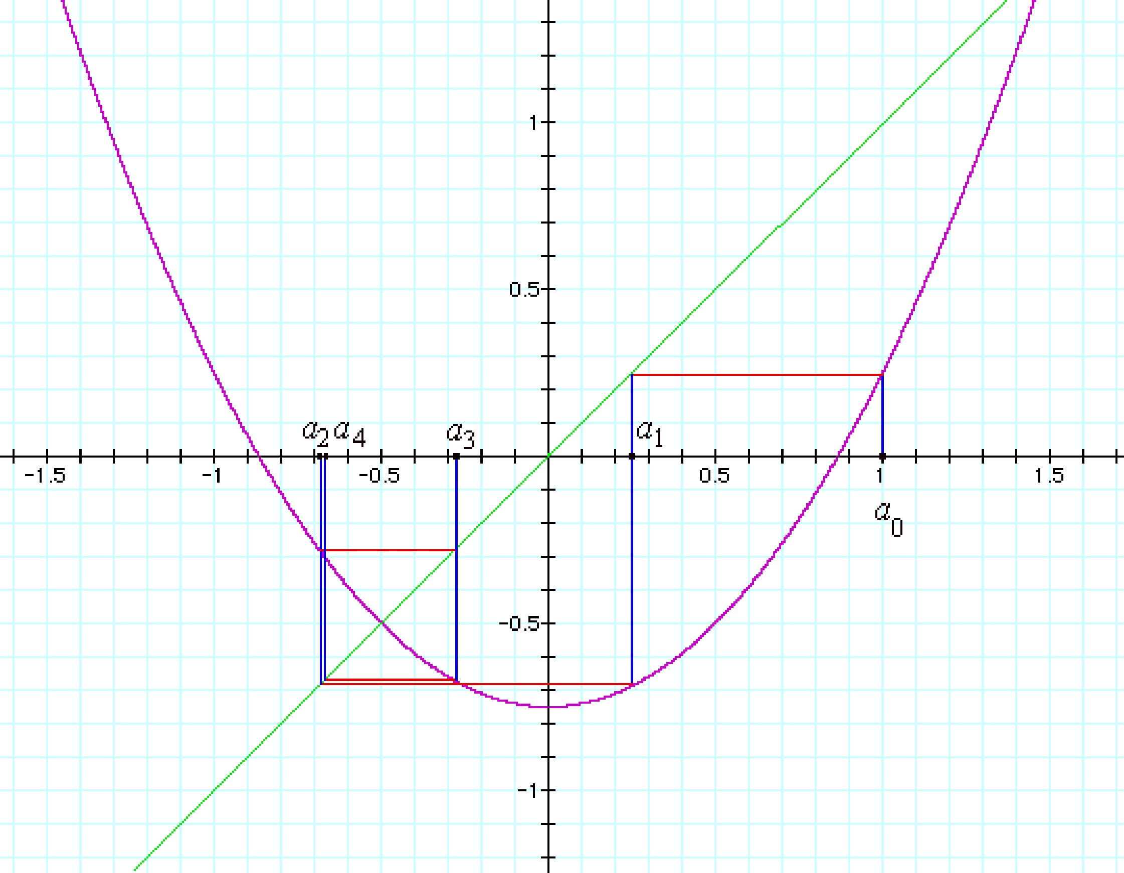
In the figure helps us to see what is happening graphically, f (x) = x^2 - 0.75 is drawn in magenta, to observe the iterations a0, a1, a2, a3 and a4 on the x-axis we draw the line y = x of green, note that to find "an + 1" from From "an" is drawn a vertical blue line of "an" to f (x) (The curve in magenta), then a horizontal line from red to green straight y = x and finally a vertical blue line back to X axis. In this way we can say that a5 is very close to the left of a3, if we make the rest of the iterations we obtain a rectangular spiral on the point where f (x) and y = x are Intercept, this puto is (-0.5, -0.5), thus, the iterations are close to -0.5.
With another initial value, for example a0 = 2, we have the following:
A0 = 2
A1 = f (2) = 42 - 0.75 = 3.25
A2 = f (3.25) = 3.252 - 0.75 = 9.8125
A3 = f (9.8125) = (9.8125) 2 = 0.75 = 95.535
A4 = f (95.535) = (95.535) 2 = 0.75 = 9126.2
A5 = f (9126.2) = (9126.2) 2 = 0.75 = 83287819.2
Note that for this case the iterations escape to infinity. Consequently those that occur with {ak: k ∈ N} depends on the initial point a0. For this case in general we have to:
If a0> 1.5 then {ak: k ∈ N} escapes to infinity.
If a0 <-1.5 then a1> 1.5 therefore {ak: k ∈ N} escapes to infinity.
If -1.5 <a0 <1.5 then {ak: k ∈ N} approaches -0.5.
If a0 = -1.5 'or a0 = 1.5 then {ak: k ∈ N} approaches 1.5.
Note that the real line has been partitioned into three sets; The closed interval [-1.5; 1.5] where {ak: k ∈ N} remains bounded if a0 is in that interval and the open intervals (-∞; -1.5) and (1,5; ∞) in which {ak: k ∈ N} escapes to infinity if a0 belongs to them. To the sets of the initial points whose iterations remain bounded we will call it the sets of Julia.
enjoy, resteem and follow me @falcao12
Much mathematic and figures. Good job
Thanks my friend!